Trading on Quantum Mechanics: How to Build an Autonomous AI Agent

The same math that describes a particle in two places at once can describe a portfolio in two positions at once. Here is how to turn the structure of quantum mechanics into an autonomous trading agent - and, just as important, where the analogy stops being real and starts being marketing.

1. Why quantum, and why now

Every hedge fund on the planet is grinding the same three ideas into dust: momentum, mean-reversion, and some flavor of machine learning on order-flow. The edge keeps thinning because the model of the market everyone shares is identical - a classical one, where a price is a single number and the future is a single noisy path.

Quantum mechanics offers a different data model. A quantum system is never in one state. It lives in a superposition of all possible states at once, each carrying a complex probability amplitude. That happens to be a strikingly good description of a market before you place a trade: the asset is simultaneously going up, going down, and chopping sideways, each outcome weighted by a probability, until your order forces reality to pick one.

Here is the part most threads skip, so let me put it up front. You do not need a physical quantum computer for any of this, and most of what follows is not literally quantum. It is quantum-inspired: classical algorithms that borrow the mathematical structure of quantum mechanics - state vectors, complex amplitudes, Hamiltonians, annealing, interference - and run on the same GPU you already own. The value is in the structure, not in qubits. Being honest about that distinction is what separates a usable framework from a buzzword.

Banks and quant shops - Goldman Sachs, JPMorgan, HSBC, and specialists like Multiverse Computing among them - have actively researched and published on quantum and quantum-inspired methods for derivative pricing, Monte Carlo risk, and portfolio optimization. The theory is public. What almost nobody has written down is how to wire it into an autonomous agent - a system that perceives, decides, executes, and learns on its own. That is what we build here.

2. The quantum-to-market dictionary

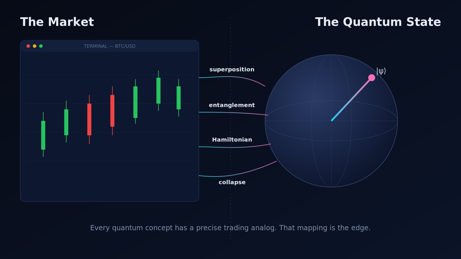
Before any code, you need the mapping. Each quantum concept below has a precise trading analog. Treat this section as the conceptual contract for everything that follows.

Probability amplitude maps to conviction - but with a phase. Classical probabilities are just non-negative numbers. Quantum amplitudes are complex: each carries a magnitude and a phase angle. Phase is the entire upgrade. It is what lets two bullish signals destructively interfere and cancel, or two weak signals constructively interfere into a strong one. A classical ensemble that averages positive probabilities physically cannot do this - the best it can do is dilute. Phase lets signals actively veto each other.

Entanglement maps to correlation you cannot factor apart. When two assets move as a linked regime - think a majorcoin and the memecoins that ride its liquidity - you cannot honestly describe one without the other. The agent encodes this as a non-separable state, which captures regime-linked co-movement that a static correlation matrix tends to flatten and understate, especially in the tails.

The Hamiltonian maps to your risk/return cost function. In physics, the Hamiltonian H encodes a system's energy. In trading, you encode your objective - maximize expected return, minimize variance, respect position and budget limits - as an energy landscape. The optimal portfolio is then the ground state: the lowest-energy configuration of H. Portfolio construction becomes an energy-minimization problem, which is a very well-studied thing to solve.

Measurement and collapse map to execution. The instant you send an order, the superposition collapses to one realized outcome. The agent's real job is to choose when and what to measure so the collapse tends to land on a profitable configuration. There is even a built-in risk principle by analogy to Heisenberg: you cannot simultaneously pin down a position's exact price and its exact momentum with unlimited precision. Demanding more certainty on one costs you certainty on the other. This is an analogy, not a law of finance - but it is a useful one, and later it turns into a concrete position-sizing rule.

3. The architecture of a quantum trading agent

The agent is a closed loop of six modules. The architecture diagram attached to this post shows the full cycle; here is what each stage does.

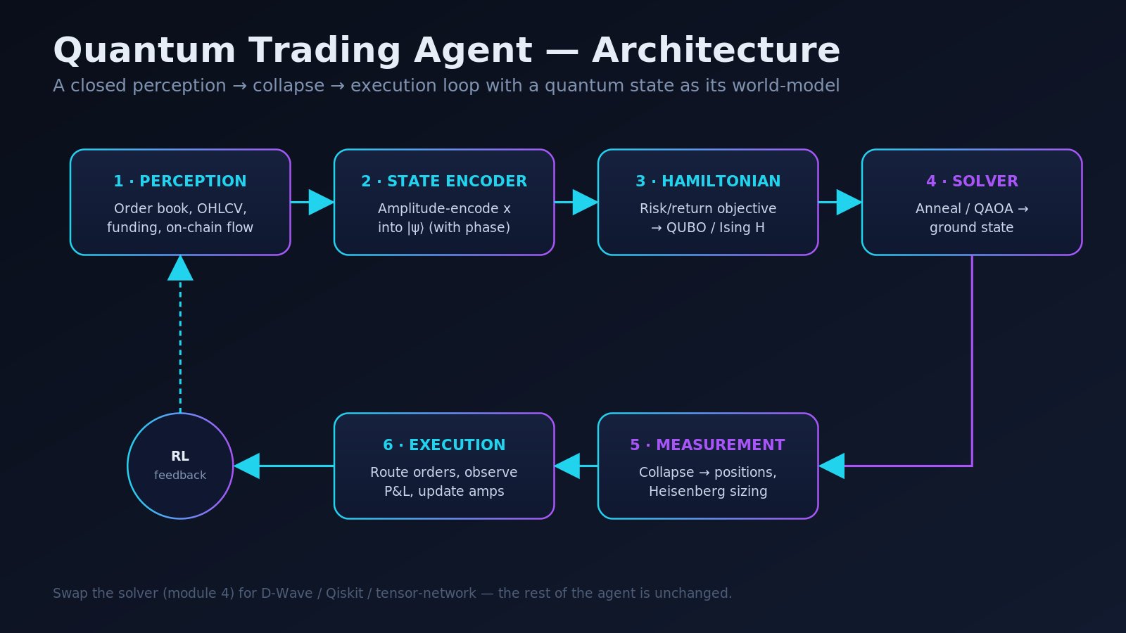
1. Perception. Ingest raw market data - order book, OHLCV, funding rates, on-chain flow. Normalize it into a feature vector x. This is ordinary quant plumbing; nothing quantum yet.

3. Hamiltonian builder. Translate your risk/return objective plus constraints into a QUBO / Ising Hamiltonian H. This is where budget limits, risk aversion, and expected returns get baked into an energy landscape.

4. Quantum-inspired solver. Find the ground state of H - the optimal asset selection - via simulated annealing, a QAOA circuit on a simulator, or a tensor-network solver. This module is your portfolio optimizer, and it is deliberately swappable.

5. Decision by measurement. Collapse the state into concrete positions and sizes, with the Heisenberg-style rule shrinking exposure when uncertainty is high.

6. Execution and feedback. Route the orders, observe realized P&L, and update the amplitudes. The measured outcome becomes tomorrow's prior - a reinforcement loop that lets the agent adapt instead of running a frozen strategy.

4. Code: encoding the market as a quantum state

We will use numpy for the state math and lean on qiskit / pennylane conventions for the quantum-inspired parts. Nothing here needs real quantum hardware - it runs on a laptop.

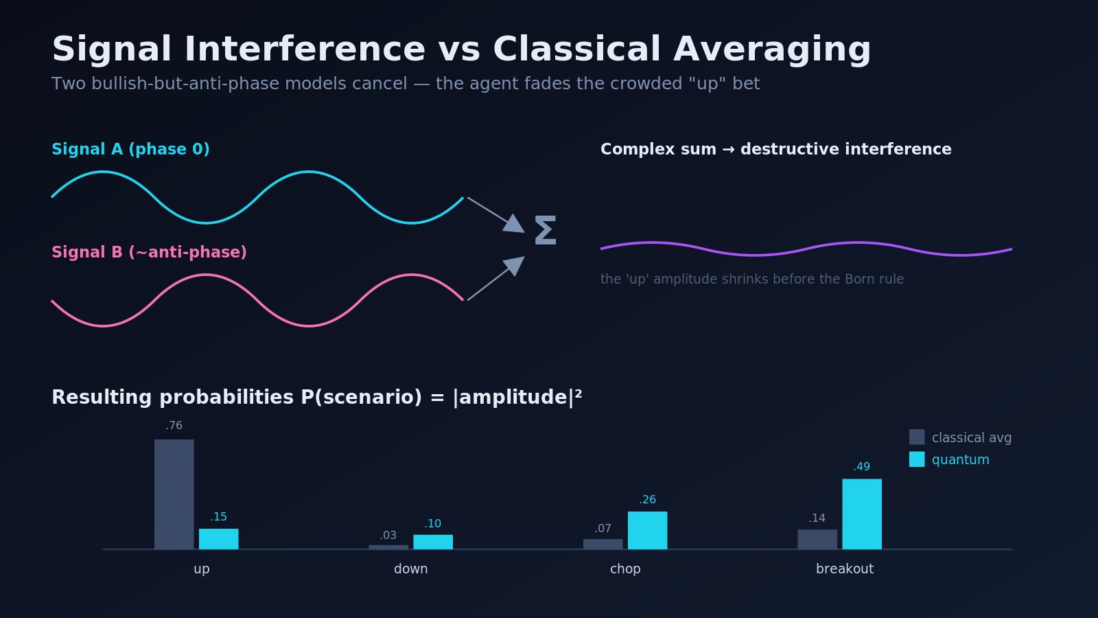
Interference is the whole point, so the encoding must let signals add as complex numbers before you take probabilities. Each alpha model contributes a complex amplitude - magnitude equals conviction, phase equals timing or regime alignment - to each market scenario. You sum the contributions across models, and only then apply the Born rule.

1import numpy as np
2
3def combine_signals(contributions: np.ndarray) -> np.ndarray:
4    """
5    contributions: complex matrix of shape [n_signals, n_scenarios].
6                   |value| = a model's conviction for a scenario,
7                   angle   = its phase (timing / regime alignment).
8    returns:       normalized state |psi> over the scenarios.
9    """
10    amplitudes = contributions.sum(axis=0)          # signals INTERFERE here
11    return amplitudes / np.linalg.norm(amplitudes)
12
13# Scenarios: [up, down, chop, breakout]
14# Two momentum models both lean 'up' -- but they are out of phase, so they partly cancel.
15signal_A = np.array([0.7+0j, 0.1+0j, 0.2+0j, 0.3+0j])       # bullish, phase 0
16signal_B = np.array([0.6*np.exp(1j*2.7), 0.15, 0.2, 0.25])  # bullish but ~anti-phase
17
18psi = combine_signals(np.vstack([signal_A, signal_B]))
19
20# Probability of each scenario = |amplitude|^2  (the Born rule)
21probs = np.abs(psi) ** 2
22print(probs.round(3))   # -> [0.147 0.102 0.26 0.491]

The key line is the Born rule: probability equals the squared magnitude of the amplitude. Because the two bullish signals are summed as complex numbers before squaring, their out-of-phase components cancel, and the crowded "up" scenario is suppressed from a naive 0.76 down to 0.147. The agent automatically fades an over-correlated consensus bet. That is the concrete, measurable difference between this and a plain probability-averaging ensemble, and the interference diagram attached to this post shows the same numbers side by side.

5. The hard part nobody shows you: where does the phase come from?

Every thread that sells you "quantum trading" quietly hard-codes the phases and hopes you do not notice. In the snippet above I wrote np.exp(1j\2.7) by hand. In a real system, inventing the phase is the entire research problem*, and pretending otherwise is the fastest way to fool yourself.

So treat phase as a first-class modeling target, not a decoration. A few grounded ways to derive it instead of guessing:

Timing / cycle phase. Run each signal through a Hilbert transform or a wavelet decomposition and read off the instantaneous phase of the dominant cycle. Two momentum models that fire on the same direction but on different cycle phases genuinely should partially cancel - that is exactly the crowding you want to detect.

Lead-lag phase. Estimate the cross-correlation lag between a signal and forward returns. Convert that lag into an angle. Signals that lead price get one phase; laggards that are really just chasing get another, so they interfere destructively with the leaders instead of double-counting.

Regime phase. Map a regime classifier (trend vs range, high vs low vol) onto an angle so that a signal's contribution rotates as the regime rotates. A breakout model and a mean-reversion model then naturally sit near opposite phases.

The discipline is simple: if you cannot explain why a signal has the phase it has, you do not get to use phase. Fall back to phase 0 for everything, and you are back to a classical ensemble - which is fine and honest. Phase is powerful precisely because it is hard-won.

6. Code: the portfolio as a ground-state search

Portfolio selection under constraints is combinatorial optimization - pick the best subset of assets subject to a budget and risk limits. That is exactly the shape of problem annealing was built for. We encode "which assets to hold" as a QUBO (Quadratic Unconstrained Binary Optimization), the classical twin of an Ising Hamiltonian.

1import numpy as np
2
3def build_portfolio_hamiltonian(expected_returns, cov, risk_aversion=1.0,
4                                budget=3, penalty=5.0):
5    """
6    Build a QUBO matrix Q so that minimizing x^T Q x  (x in {0,1}^n)
7    picks the best 'budget' assets: maximize return, minimize risk,
8    and softly penalize breaking the budget constraint.
9    """
10    n = len(expected_returns)
11    Q = np.zeros((n, n))
12
13    # return (negated, since we minimize) plus a risk term from the covariance
14    for i in range(n):
15        Q[i, i] += -expected_returns[i] + risk_aversion * cov[i, i]
16        for j in range(i + 1, n):
17            Q[i, j] += 2 * risk_aversion * cov[i, j]
18
19    # budget constraint (sum x_i - budget)^2 as a soft penalty
20    for i in range(n):
21        Q[i, i] += penalty * (1 - 2 * budget)
22        for j in range(i + 1, n):
23            Q[i, j] += 2 * penalty
24    return Q
25
26def simulated_anneal(Q, steps=20000, T0=5.0):
27    """Quantum-inspired annealing: slowly cool the system into its ground state."""
28    n = Q.shape[0]
29    x = np.random.randint(0, 2, n)
30    def energy(x): return x @ Q @ x
31    e = energy(x)
32    for t in range(steps):
33        T = T0 * (1 - t / steps)                 # linear temperature schedule
34        i = np.random.randint(n)
35        x_new = x.copy(); x_new[i] ^= 1          # flip one asset in/out
36        e_new = energy(x_new)
37        # accept improvements always, and worse moves sometimes (that is how it escapes local minima)
38        if e_new < e or np.random.rand() < np.exp(-(e_new - e) / max(T, 1e-9)):
39            x, e = x_new, e_new
40    return x, e
41
42returns = np.array([0.12, 0.09, 0.15, 0.04, 0.11])
43cov = np.array([
44    [0.10, 0.02, 0.01, 0.00, 0.03],
45    [0.02, 0.08, 0.02, 0.01, 0.01],
46    [0.01, 0.02, 0.18, 0.00, 0.02],
47    [0.00, 0.01, 0.00, 0.03, 0.00],
48    [0.03, 0.01, 0.02, 0.00, 0.09],
49])
50Q = build_portfolio_hamiltonian(returns, cov, risk_aversion=2.0, budget=2)
51selection, ground_energy = simulated_anneal(Q)
52print("Hold assets:", np.where(selection == 1)[0], "| energy:", round(ground_energy, 3))

One honest note on scale. At five assets you do not need annealing — you could brute-force all 32 combinations. Annealing earns its keep at hundreds of assets with hard constraints, where the search space explodes and exact solvers choke. The reason to write it this way at small scale is that the interface never changes: swap simulated_anneal for a real backend — D-Wave's annealer, a QAOA circuit on a Qiskit simulator, or a tensor-network solver of the kind Multiverse ships — and nothing else in the agent moves. The solver is a plug.

7. Code: the agent loop (perception to collapse to execution)

Now wire it together. This is the skeleton of an autonomous agent - the same perceive/decide/act control loop an LLM agent uses, but with a quantum-style state as its world-model instead of text.

1class QuantumTradingAgent:
2    def __init__(self, universe, risk_aversion=2.0, budget=2, gross_leverage=1.0):
3        self.universe = universe
4        self.risk_aversion = risk_aversion
5        self.budget = budget
6        self.gross_leverage = gross_leverage
7        self.memory = []                     # feedback / RL buffer
8
9    def perceive(self, market):
10        contributions = self.model_conviction(market)   # your alpha models -> complex matrix
11        return combine_signals(contributions)            # -> state |psi> over scenarios
12
13    def deliberate(self, market):
14        Q = build_portfolio_hamiltonian(
15            market["expected_returns"], market["cov"],
16            self.risk_aversion, self.budget)
17        selection, _ = simulated_anneal(Q)
18        return selection
19
20    def measure(self, psi, selection, market):
21        """
22        Collapse into orders. Two things happen here:
23        1) a GLOBAL conviction gate from the scenario state (directional + Heisenberg vol shrink)
24        2) a PER-ASSET weight so the chosen assets are sized by their own expected return
25        """
26        scenario_probs = np.abs(psi) ** 2
27        directional = scenario_probs[0] + scenario_probs[3]      # P(up) + P(breakout)
28        vol = market["volatility"]
29        gate = directional / (1.0 + self.risk_aversion * vol)   # shrink in high vol / low conviction
30
31        idx = np.where(selection == 1)[0]
32        if len(idx) == 0:
33            return {}
34        edge = np.clip(market["expected_returns"][idx], 0, None) # only long positive-edge names
35        weights = edge / edge.sum() if edge.sum() > 0 else np.ones(len(idx)) / len(idx)
36
37        sizes = self.gross_leverage * gate * weights
38        return {int(a): round(float(s), 4) for a, s in zip(idx, sizes)}
39
40    def act(self, market):
41        psi = self.perceive(market)
42        selection = self.deliberate(market)
43        orders = self.measure(psi, selection, market)
44        # execute(orders)   <- route to exchange / broker here
45        self.memory.append((market, orders))
46        return orders

Look closely at measure(), because the earlier naive version had a real flaw: it applied one identical size to every selected asset, ignoring how good each one actually was. This version fixes it with two stages. A global gate reads the scenario state - directional conviction, which is P(up) + P(breakout), divided by a volatility term. That division is the Heisenberg-style rule doing risk management: the more the market resists precise pricing, meaning higher volatility, the smaller the agent's total commitment. Then a per-asset weight distributes that budget across the selected names in proportion to their own expected edge, and refuses to long anything with negative expected return. Conviction sets how much you bet; per-asset edge sets where it goes.

8. The Wall Street reality check

Where does this actually earn money, and where is it a beautiful demo? Being specific here is what makes the rest credible.

Genuine edge today, on classical hardware:

Portfolio optimization at scale. With hundreds of assets and hard constraints, annealers and tensor-network methods handle the combinatorics and the constraints more gracefully than naive mean-variance solvers, and often faster. This is the most mature, least hype-prone application.

Risk estimation via quantum amplitude estimation. In theory this offers a quadratic speedup over classical Monte Carlo for VaR and CVaR. It remains one of the most actively researched directions at large banks, because risk runs are expensive and run constantly. Note the caveat: the headline speedup is a theoretical asymptotic result, and today's hardware does not yet realize it at production scale.

Signal combination via interference. Modeling conviction with a phase so that crowded, over-correlated trades cancel is a genuinely useful reframing, and it works on your existing GPU today. It is the most immediately practical idea in this article - provided you solve the phase problem from Section 5 honestly.

Still mostly research:

End-to-end derivative pricing on real quantum hardware. Promising in principle, but noise and qubit counts limit it today.

"Quantum ML" price prediction. Heavily over-hyped. The cost of loading classical market data into a quantum state usually eats any speedup you hoped to gain. Be very skeptical of anyone selling this.

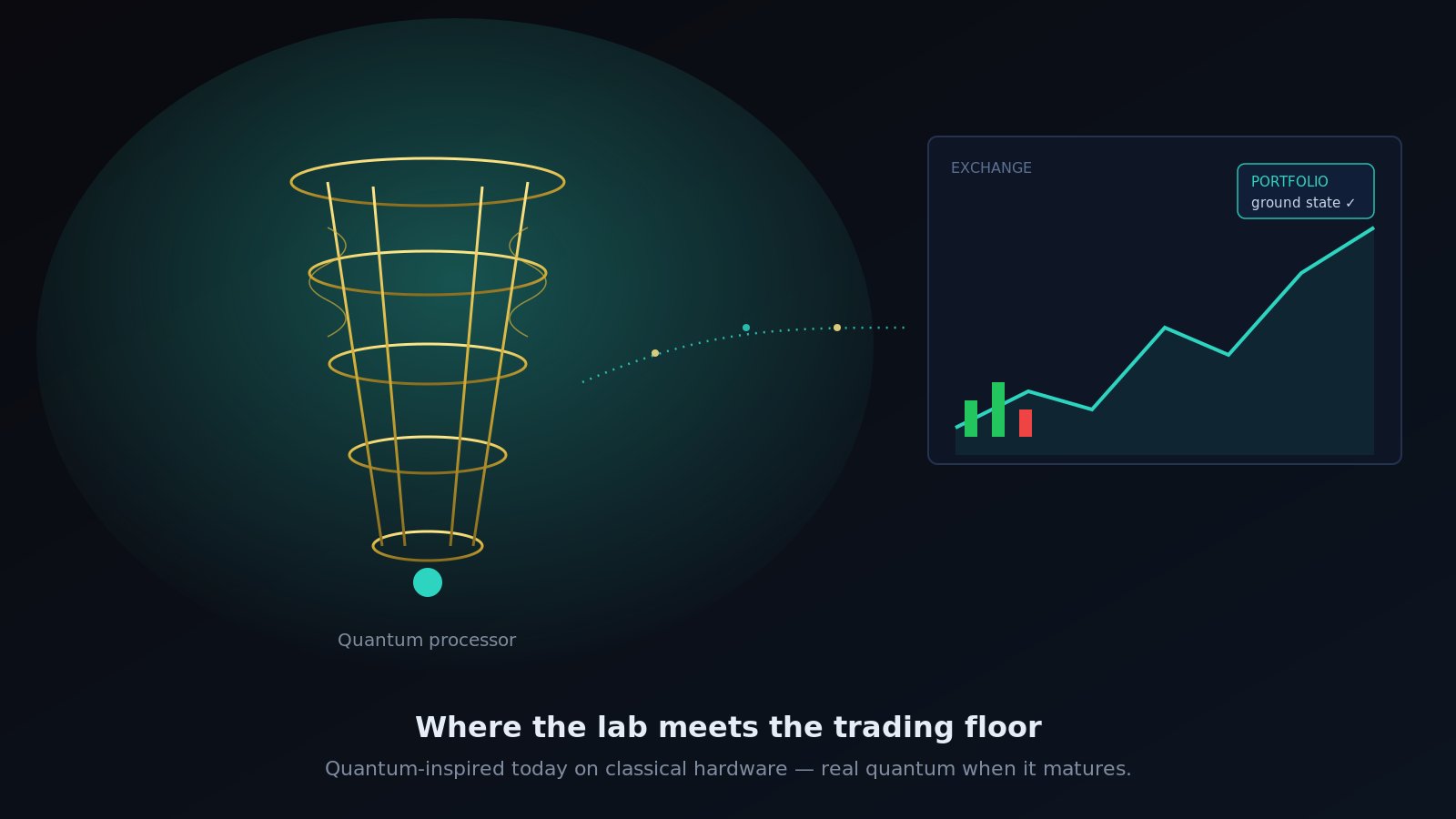
The honest bottom line: the quantum-inspired agent is buildable and backtestable right now, because every module runs on classical hardware. You capture the structural ideas - a superposition of hypotheses, destructive interference against crowding, Hamiltonian-based optimization - without waiting for fault-tolerant quantum computers. When the hardware matures, you swap module 4 and keep the rest.

9. What will actually kill this in production

Every strategy looks brilliant until it meets the market. Before you risk a dollar, internalize the four things that quietly destroy quantum-inspired agents specifically.

Transaction costs and slippage. The interference layer reshuffles conviction every time new data arrives, which tempts the agent to churn its book. Fees and slippage do not care how elegant your state vector is. Add a turnover penalty directly into the Hamiltonian and re-run - many "edges" evaporate the moment realistic costs are charged.

Overfitting the phases. Phase gives you a whole extra set of free parameters, and free parameters are how backtests lie. It is trivially easy to tune phases until last year prints money and next year bleeds. Fix the phase rules from theory (Section 5) before you look at returns, and never let the backtest choose them for you.

Data-snooping across the loop. Because this is a closed feedback loop, leakage compounds. If your conviction model, your covariance estimate, or your regime labels peek even slightly into the future, the whole agent inherits the lie. Walk-forward test the entire loop, not just the signal in isolation.

Regime fragility of the covariance. The QUBO leans on a covariance matrix, and covariances blow up exactly when you need them - in a crash, correlations rush to one. Stress-test the ground-state selection under a shocked covariance, not just the calm-market one, or the optimizer will happily hand you a portfolio that is diversified only on paper.

10. Your build checklist

If you want to actually ship this, here is the order of operations.

Start with the quantum-inspired solver - plain numpy plus simulated annealing. No hardware, no accounts, no dependencies.

Replace the hand-tuned amplitudes with a learned conviction model feeding combine_signals, and derive the phases from theory rather than fitting them.

Backtest the whole loop, with costs, not just the signal. Charge realistic fees and slippage, add a turnover penalty, and walk it forward. The interference and sizing logic is where both the edge and the self-deception hide.

Only after the abstraction has paid for itself in simulation should you reach for a real backend - Qiskit or PennyLane simulator first, then D-Wave, then hardware. Swapping module 4 is a one-line change by design.

The market was always a probability wave. Almost everyone still trades it like a single number - and the gap between those two views is the whole opportunity.

If this rewired how you think about markets, repost the top and follow. The full open-source agent repo drops next. ⚛️

Disclaimer. Not financial advice, and not a promise of returns. Quantum-inspired does not mean quantum-guaranteed - most of what makes this work is disciplined classical modeling wearing a quantum coat. Backtest everything with real costs; the market collapses your wavefunction whether you are ready or not.